Calculating with time
Scope
This guide demonstrates handling of time.
We repeat ever so briefly some examples are covered in more detail elsewhere.
Storage implementation: UTC under the hood.
Calculating differeneces between versions identified by
as_of-dates is simple arithmetics after retrieving a data.Interval for data retrieval and simple filtering after retrieval of the data along the time axis using time aware functionality of other libararies.
Functions along the time axis:
Resampling to other frequencies.
Sampling and aggregations (group by).
Changing types.
Moving average.
Planned extensions:
Indexing
Diff, shift, cumsum
Proper timeseries analysis and seasonal adjustment are covered by external libraries, demonstrated later in this guide (see Timeseries analysis).
The quintessential time functions work along the time axis.
Prerequisites
Note
The guide assumes that the SSB Timeseries library is installed and that a working configuration is active. See the quickstart guide for instructions to that.
The presented functionality relies on dataset.Dataset.
Other imports liketypes.SeriesType and external libraries are used only for generating the sample data.
from ssb_timeseries.dataset import Dataset
from datetime import date
from itertools import product

import numpy as np

from ssb_timeseries.sample_data import POPU06_MAIN_COUNTRIES
from ssb_timeseries.sample_data import create_df
from ssb_timeseries.sample_data import popu06
from ssb_timeseries.types import SeriesType
Generate some test data
def create_popu06_versions(
    as_of_dates: list[date],
    countries: tuple[str, ...],
    noise: float = 0.002,
    seed: int = 20251001,
):
    """Save one version of the Nordic population projections for each as-of date.

    The projections themselves are static and reproducible, so a small seeded
    perturbation is applied to give each version its own values.
    Without it every version would hold identical numbers and calculating
    between two versions would yield nothing but zeros.
    """
    base = popu06(countries=countries, start_year=2027, end_year=2046)
    generator = np.random.default_rng(seed)
    for as_of in as_of_dates:
        version = base.copy()
        for country in countries:
            jitter = 1 + noise * generator.standard_normal(len(version))
            version[country] = (
                version[country].to_numpy() * jitter
            ).round().astype("int64")
        Dataset(
            name="POPU06",
            data_type=SeriesType("AS_OF", "AT"),
            as_of_tz=str(as_of),
            data=version,
            tags={
                "source": "POPU06",
                "table": "Population projections by age and sex, total",
            },
        ).save()
We will store the population projections published in the Nordic Statistics database table
POPU06, one series per country.
The same projections are stored once per as_of-date, so that versions can be compared.
create_popu06_versions(
    as_of_dates=[date(*d) for d in product({2024, 2025}, range(1, 13), {1})],
    countries=POPU06_MAIN_COUNTRIES,
)
Element-wise arithmetic
Our dataset “POPU06” contains population projections for the Nordic countries.
Basic arithmetic may be performed on same size data:
jul = Dataset(name="POPU06", as_of_tz="2025-07-01")
feb = Dataset(name="POPU06", as_of_tz="2025-02-01")

change_from_feb_to_july = jul - feb
change_from_feb_to_july.plot()
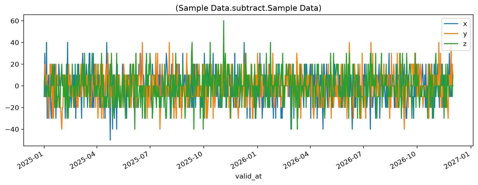
The Numpy implementation means that element-wise calculation is the default, with Numpy “broadcasting rules” for different size objects. Broadcasting rules and dimensional conditions are avaluated only for the numeric parts - the math functions will ignore the date columns. Date alignment must be performed explicitly prior to the calculation.
Narwhals under the hood first and foremost allow the arithmetic functions support operating not only on Dataset objects, but on combinations of datasets with a large number of other datatypes (scalars, Numpy arrays, dataframes, Arrow tables).
Note that the “dataframe like” objects are all conflated to ‘df’ in the lineage tracking.
Filter by dates
Narwhals also brings conversion of Dataset.data to other libraries and their functionality within short reach.
Shorthand properties Dataset.pa, .nw, .pd, and .pl return Arrow tables, and Narwhals, Pandas and Polars dataframes.
Interval support and filtering by dates is an underdeveloped area of functionality.
import polars as pl

d_from = date(2035, 1, 1)
d_to = pl.date(2039, 12, 31)
x_row = jul.pl.filter( pl.col("valid_at").is_between(d_from, d_to) )
x_row
valid_at |
Denmark |
Finland |
Iceland |
Norway |
Sweden |
|---|---|---|---|---|---|
datetime[ns, UTC] |
f64 |
f64 |
f64 |
f64 |
f64 |
2035-12-31 23:00:00 UTC |
6.134939e6 |
5.899144e6 |
468533.0 |
5.908382e6 |
1.0749026e7 |
2036-12-31 23:00:00 UTC |
6.140989e6 |
5.921987e6 |
476381.0 |
5.95139e6 |
1.0811669e7 |
2037-12-31 23:00:00 UTC |
6.130022e6 |
5.944316e6 |
479762.0 |
5.937953e6 |
1.0844831e7 |
2038-12-31 23:00:00 UTC |
6.157238e6 |
5.978206e6 |
487794.0 |
5.956446e6 |
1.0855639e7 |
# bigger example - not needed?
tags = {“Var”: [“price”, “volume”],
“Product”: [“milk”, “eggs”, “bread”, “cheese”, “ham”],
“Store”: [“A”, “B”, “C”, “D”, “E”],
“Region”: [“N”, “S”, “E”, “W”, “NE”, “NW”, “SE”, “SW”]}
some_data = create_df( *[value for value in tags.values()], start_date=”2000-12-01”, end_date=”2024-01-01”, freq=”MS”, implementation=”pandas”).set_index(‘valid_at’) some_data.info()
Resample
Dataset.resample alters the frequency of the data itself.
Upsampling to a higher frequency fills in the missing periods with a fill method, ffill or bfill.
Downsampling to a lower frequency aggregates the periods with one of the simple aggregations listed in the reference
(min, max, sum, mean, median, std, var, count, first, last).
yearly_to_daily = jul.resample("D", "ffill")
Forward fill carries each annual projection forward day by day until the next annual value arrives.
Backward fill (bfill) instead lets the next annual value populate the days before it; it suits calendars where the time point marks the end of a period.
Downsampling the daily data again averages the values inside each new period.
It reproduces the annual levels closely, but not exactly at the boundaries, because the daily grid and the annual time points do not coincide.
daily_to_yearly = yearly_to_daily.resample("YE", "mean")
daily_to_yearly.data
valid_at |
Denmark |
Finland |
Iceland |
Norway |
Sweden |
|---|---|---|---|---|---|
2027-12-30 23:00:00+00:00 |
5999359.0 |
5672363.0 |
406313.0 |
5669951.0 |
10615636.0 |
2028-12-30 23:00:00+00:00 |
5996705.0 |
5721457.0 |
412917.0 |
5684376.0 |
10625613.0 |
2029-12-30 23:00:00+00:00 |
6027401.0 |
5716670.0 |
420793.0 |
5716418.0 |
10611853.0 |
2030-12-30 23:00:00+00:00 |
6080182.0 |
5771599.0 |
427802.0 |
5722952.0 |
10591888.0 |
2031-12-30 23:00:00+00:00 |
6050448.0 |
5766510.0 |
434670.0 |
5758831.0 |
10596849.0 |
… |
… |
… |
… |
… |
… |
2042-12-30 23:00:00+00:00 |
6183954.0 |
5987105.0 |
503685.0 |
6036619.0 |
10964012.0 |
2043-12-30 23:00:00+00:00 |
6182232.0 |
6049960.0 |
506589.0 |
6043889.0 |
11004110.0 |
2044-12-30 23:00:00+00:00 |
6208393.0 |
6045014.0 |
512525.0 |
6072128.0 |
11013343.0 |
2045-12-30 23:00:00+00:00 |
6170663.0 |
6063181.0 |
519735.0 |
6085844.0 |
11114163.0 |
2046-12-30 23:00:00+00:00 |
6195530.0 |
6089520.0 |
521892.0 |
6106436.0 |
11117373.0 |
Group by
Dataset.group_by aggregates over calendar periods rather than changing the frequency.
freq is an alias enumerated in the group_by reference, with the same meaning on all backends:
year (y/yr), month (m/mth), quarter (q), week (w/wk), or raw for already-formatted values.
func may be a function name or a list of function names that apply to every series, or agg_mapping may map functions to specific series; tz converts the time column before grouping, and time_col picks the column to group on.
jul.pl.describe().select(pl.col(["statistic", "valid_at"]))
statistic |
valid_at |
|---|---|
str |
str |
“count” |
“20” |
“null_count” |
“0” |
“mean” |
“2036-07-01 23:00:00+00:00” |
“std” |
null |
“min” |
“2026-12-31 23:00:00+00:00” |
“25%” |
“2031-12-31 23:00:00+00:00” |
“50%” |
“2036-12-31 23:00:00+00:00” |
“75%” |
“2040-12-31 23:00:00+00:00” |
“max” |
“2045-12-31 23:00:00+00:00” |
weekly = yearly_to_daily.group_by("week", "mean")
weekly.data.head(6)
valid_at |
Denmark_week_mean |
Finland_week_mean |
Iceland_week_mean |
Norway_week_mean |
Sweden_week_mean |
|---|---|---|---|---|---|
2026-53 |
5999359.0 |
5672363.0 |
406313.0 |
5669951.0 |
10615636.0 |
2027-01 |
5999359.0 |
5672363.0 |
406313.0 |
5669951.0 |
10615636.0 |
2027-02 |
5999359.0 |
5672363.0 |
406313.0 |
5669951.0 |
10615636.0 |
2027-03 |
5999359.0 |
5672363.0 |
406313.0 |
5669951.0 |
10615636.0 |
2027-04 |
5999359.0 |
5672363.0 |
406313.0 |
5669951.0 |
10615636.0 |
2027-05 |
5999359.0 |
5672363.0 |
406313.0 |
5669951.0 |
10615636.0 |
quarterly = yearly_to_daily.group_by("quarter", "mean", tz="Europe/Oslo")
quarterly.data.head(6)
valid_at |
Denmark_quarter_mean |
Finland_quarter_mean |
Iceland_quarter_mean |
Norway_quarter_mean |
Sweden_quarter_mean |
|---|---|---|---|---|---|
2027-Q1 |
5999359.0 |
5672363.0 |
406313.0 |
5669951.0 |
10615636.0 |
2027-Q2 |
5999359.0 |
5672363.0 |
406313.0 |
5669951.0 |
10615636.0 |
2027-Q3 |
5999359.0 |
5672363.0 |
406313.0 |
5669951.0 |
10615636.0 |
2027-Q4 |
5999359.0 |
5672363.0 |
406313.0 |
5669951.0 |
10615636.0 |
2028-Q1 |
5996705.0 |
5721457.0 |
412917.0 |
5684376.0 |
10625613.0 |
2028-Q2 |
5996705.0 |
5721457.0 |
412917.0 |
5684376.0 |
10625613.0 |
Moving average
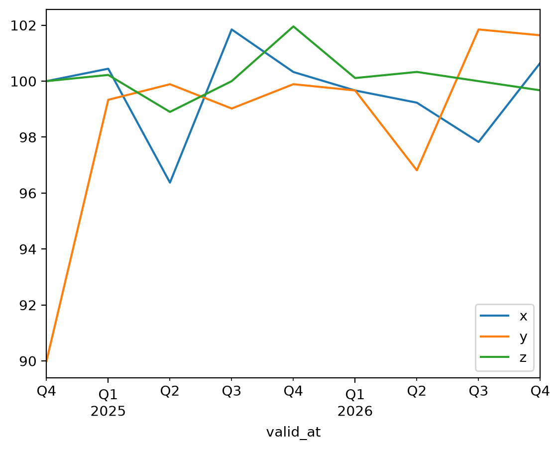
four_week_average = weekly.moving_average(-3, 0)
four_week_average.data
pyarrow.Table
valid_at: string
Denmark_week_mean: double
Finland_week_mean: double
Iceland_week_mean: double
Norway_week_mean: double
Sweden_week_mean: double
----
valid_at: [["2026-53","2027-01","2027-02","2027-03","2027-04",...,"2045-49","2045-50","2045-51","2045-52","2046-01"]]
Denmark_week_mean: [[nan,nan,nan,5999359,5999359,...,6170663,6170663,6170663,6170663,6176879.75]]
Finland_week_mean: [[nan,nan,nan,5672363,5672363,...,6063181,6063181,6063181,6063181,6069765.75]]
Iceland_week_mean: [[nan,nan,nan,406313,406313,...,519735,519735,519735,519735,520274.25]]
Norway_week_mean: [[nan,nan,nan,5669951,5669951,...,6085844,6085844,6085844,6085844,6090992]]
Sweden_week_mean: [[nan,nan,nan,10615636,10615636,...,11114163,11114163,11114163,11114163,11114965.5]]
four_week_average.pd.plot()
Timeseries analysis
Proper time series analysis and seasonal adjustment are beyond the scope of the library itself.
SSB Timeseries manages storage, versioning and retrieval of the series, and defers the analysis to specialised libraries from the Python ecosystem:
Nixtla, Darts, statsmodels and Prophet are common choices.
The interoperability guide collects the available data exchange surfaces.
The frame adapters, including nixtla(), live on the Series objects that iteration over a Dataset yields.
from statsforecast import StatsForecast
from statsforecast.models import AutoARIMA
norway_series = next(s for s in jul if s.name == "Norway")
forecast = StatsForecast(
    models=[AutoARIMA(season_length=1)],
    freq="YE",
).forecast(df=norway_series.nixtla(), h=5)
nixtla() returns the Nixtla long format (unique_id, ds, y), one table per series.
Forecasts for several series can be combined by iterating the Dataset and calling nixtla() for each Series in turn.
forecast
unique_id |
ds |
AutoARIMA |
|---|---|---|
POPU06::Norway |
2046-12-31 23:00:00+00:00 |
6.133891e+06 |
POPU06::Norway |
2047-12-31 23:00:00+00:00 |
6.157177e+06 |
POPU06::Norway |
2048-12-31 23:00:00+00:00 |
6.180462e+06 |
POPU06::Norway |
2049-12-31 23:00:00+00:00 |
6.203748e+06 |
POPU06::Norway |
2050-12-31 23:00:00+00:00 |
6.227033e+06 |
See also Calculating with time or Calculating with metadata.