Read an Arrow multi-file dataset and create sf object

Read an Arrow multi-file dataset and create sf object

Usage

read_sf_dataset(dataset, find_geom = FALSE)

Arguments

dataset

a Dataset object created by arrow::open_dataset or an arrow_dplyr_query

find_geom

logical. Only needed when returning a subset of columns. Should all available geometry columns be selected and added to to the dataset query without being named? Default is FALSE to require geometry column(s) to be selected specifically.

Value

object of class sf

Details

This function is primarily for use after opening a dataset with arrow::open_dataset. Users can then query the arrow Dataset using dplyr methods such as filter or select. Passing the resulting query to this function will parse the datasets and create an sf object. The function expects consistent geographic metadata to be stored with the dataset in order to create sf objects.

See also

open_dataset, st_read, st_read_parquet

Examples

# read spatial object
nc <- sf::st_read(system.file("shape/nc.shp", package="sf"), quiet = TRUE)

# create random grouping
nc$group <- sample(1:3, nrow(nc), replace = TRUE)

# use dplyr to group the dataset. %>% also allowed
nc_g <- dplyr::group_by(nc, group)

# write out to parquet datasets
tf <- tempfile()  # create temporary location
on.exit(unlink(tf))
# partitioning determined by dplyr 'group_vars'
write_sf_dataset(nc_g, path = tf)

list.files(tf, recursive = TRUE)
#> [1] "group=1/part-0.parquet" "group=2/part-0.parquet" "group=3/part-0.parquet"

# open parquet files from dataset
ds <- arrow::open_dataset(tf)

# create a query. %>% also allowed
q <- dplyr::filter(ds, group == 1)

# read the dataset (piping syntax also works)
nc_d <- read_sf_dataset(dataset = q)

nc_d
#> Simple feature collection with 36 features and 15 fields
#> Geometry type: MULTIPOLYGON
#> Dimension:     XY
#> Bounding box:  xmin: -84.32385 ymin: 34.30457 xmax: -75.45698 ymax: 36.58965
#> Geodetic CRS:  NAD27
#> First 10 features:
#>     AREA PERIMETER CNTY_ CNTY_ID       NAME  FIPS FIPSNO CRESS_ID BIR74 SID74
#> 1  0.114     1.442  1825    1825       Ashe 37009  37009        5  1091     1
#> 2  0.143     1.630  1828    1828      Surry 37171  37171       86  3188     5
#> 3  0.097     1.670  1833    1833   Hertford 37091  37091       46  1452     7
#> 4  0.114     1.352  1838    1838    Caswell 37033  37033       17  1035     2
#> 5  0.153     1.616  1839    1839 Rockingham 37157  37157       79  4449    16
#> 6  0.072     1.085  1842    1842      Vance 37181  37181       91  2180     4
#> 7  0.190     2.204  1846    1846    Halifax 37083  37083       42  3608    18
#> 8  0.111     1.392  1904    1904   Alamance 37001  37001        1  4672    13
#> 9  0.059     1.319  1927    1927   Mitchell 37121  37121       61   671     0
#> 10 0.122     1.516  1932    1932   Caldwell 37027  37027       14  3609     6
#>    NWBIR74 BIR79 SID79 NWBIR79 group                       geometry
#> 1       10  1364     0      19     1 MULTIPOLYGON (((-81.47276 3...
#> 2      208  3616     6     260     1 MULTIPOLYGON (((-80.45634 3...
#> 3      954  1838     5    1237     1 MULTIPOLYGON (((-76.74506 3...
#> 4      550  1253     2     597     1 MULTIPOLYGON (((-79.53051 3...
#> 5     1243  5386     5    1369     1 MULTIPOLYGON (((-79.53051 3...
#> 6     1179  2753     6    1492     1 MULTIPOLYGON (((-78.49252 3...
#> 7     2365  4463    17    2980     1 MULTIPOLYGON (((-77.33221 3...
#> 8     1243  5767    11    1397     1 MULTIPOLYGON (((-79.24619 3...
#> 9        1   919     2       4     1 MULTIPOLYGON (((-82.11885 3...
#> 10     309  4249     9     360     1 MULTIPOLYGON (((-81.32813 3...
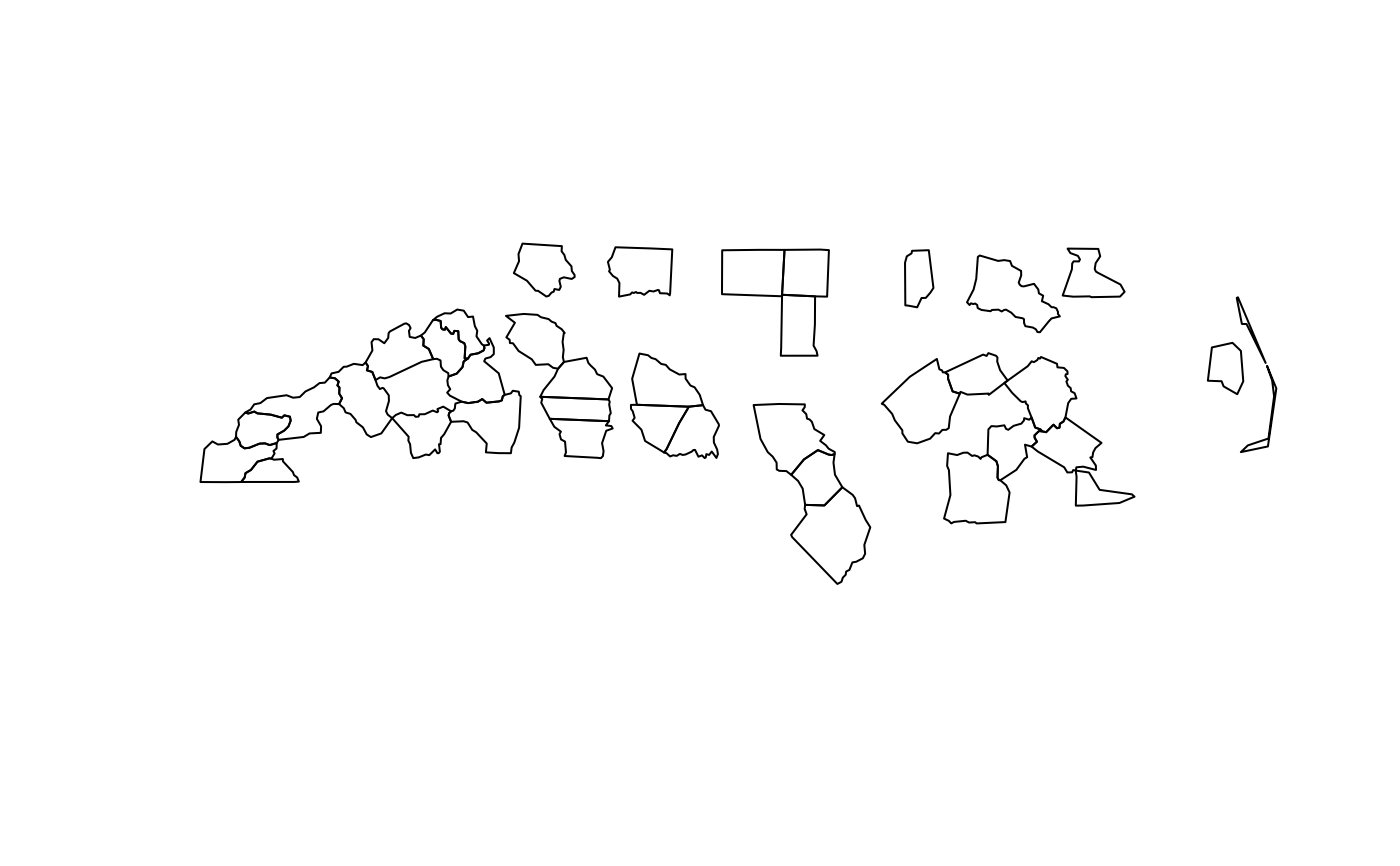
plot(sf::st_geometry(nc_d))